This section provides a brief non-technical introduction to key environmental economic concepts and principles that are relevant to LME/MPA/ICM assessment and management, including public goods, common pool resources, externalities, economic value and economic policy instruments.

2.1 Public goods and common pool resources

Goods, services and resources can be usefully defined by two characteristics: (1) excludability – the feasibility of excluding others from access and use; and (2) rivalry – the extent to which use by one person reduces the quantity available to others. To some extent, these characteristics are inherent in the nature of the good, service or resource (from hereon “goods” for short) but can also be determined by social and legal institutions.

Goods with different combinations of excludability and rivalry characteristics can be classified accordingly. Table 1 summarises the possible combinations of these characteristics to define different types of goods. Those that are excludable and rival are termed “pure private goods”. It is possible to exclude others from using such goods and consumption by one person directly reduces the quantity available to others. Examples of pure private goods are offshore fossil fuel reserves and aquaculture cages. Goods that are excludable but non-rival are termed “club goods”. An example of a club good is genetic information extracted from coral for pharmaceutical applications. Other potential users of this information can be excluded through the patent system but use of the information does not reduce the quantity available to others. Goods that are non-excludable and rival are termed “common goods” or in the case of resources, “common pool resources”. In the absence of access controls, fish stocks are examples of common pool resources in the sense that it is not feasible to exclude fishers from harvesting from the stock but their catch reduces the quantity available to other fishers. The implications for resource use and management of common pool resources is returned to later. Goods that are both non-excludable and non-rival are termed “pure public goods”. Examples include public beaches (up to the point that crowding results in rival use) and climate regulation provided by the storage of carbon in marine ecosystems. In the case of climate regulation, it is not feasible to exclude anyone from benefiting from this service and one person’s benefit from an equable climate does not reduce the benefit to anyone else.

Table 1: Combinations of excludability and rivalry characteristics used to classify different types of goods, services and resources

The characteristics of excludability and rivalry have important implications for how a good, service or resource is produced, used and managed. Open access common pool resources, including many fisheries and particularly those that have transboundary stocks or are in Areas Beyond National Jurisdiction (ABNJ), have a tendency towards overexploitation because individual users do not have an incentive to invest in maintaining the resource. This overuse of common pool resources has been eloquently described as “the tragedy of the commons” (Hardin, 1968). Chapter 8 introduces a number of policy instruments that can be used to regulate the use of common pool resources.

Pure public goods tend to be under-provided by markets (quantities are lower than socially optimal levels), unprotected by property rights, or not provided at all. The reason why private enterprises do not supply public goods is that they cannot restrict use to only those consumers who have paid for the good. In addition there is a free rider problem in that there is no incentive for consumers to pay for a good that they can obtain for free if someone else pays. In the absence of markets providing public goods there are strong arguments for governments to supply them. This requires, however, that governments know how much of a public good people want. Non-market economic valuation studies can be used to provide such information (see Chapter 6).

2.2 Externalities

The term “externality” is used to describe a negative or positive impact on the welfare of one economic agent resulting from the behaviour of another economic agent, without that impact being agreed to by the impacted party. For example, nutrient runoff from agricultural land may end up in the sea causing eutrophication and consequently damage to coastal fisheries. This is a negative externality from agricultural activities that is incurred by the fishery. An example of a positive externality is the increase in marine biodiversity resulting from the nursery function provided by offshore wind power turbines, which might be enjoyed by coastal tourists. This is a positive externality from the power producer to the tourists.

A negative externality is also called an “external cost”; and a positive externality is called an “external benefit”. In other words, these are costs and benefits that are external to the economic agent that generated them. The implication of external costs is that since the economic agents that generate the cost do not incur it themselves, they ignore it in their decision making and produce more than they otherwise would. The reverse is true for external benefits; economic agents that generate external benefits would produce more if the benefit accrued to themselves.

Externalities can be caused by both production and consumption activities; and also incurred by both producers and consumers. The above example of nutrient runoff is a production-to-production externality; and the example of wind turbines supporting marine biodiversity is a production-to-consumption externality.

Many environmental problems can be characterised as externalities. The over-exploitation of common pool resources such as fisheries is driven by an externality. An external cost is generated when one fisherman catches fish, thereby reducing the availability of fish for others to catch and increasing their costs of catching fish. Moreover, this external cost reduces the incentive for any fisherman to invest in maintaining the fish stock for future use since others can harvest any investment.

Other examples of external costs in the context of LME/MPA/ICM are other forms of marine pollution (marine plastics, oil spills, ship waste, deep sea mining), underwater noise, ocean acidification, ocean warming, and sea level rise. Chapter 6 outlines the available economic methods for valuing externalities to understand their implications for human welfare and to design policy instruments to manage them. Chapter 8 introduces a number of policy instruments that can be used to regulate externalities or internalise them so that the economic agents that generate them take them into account.

2.3 Economic value

Economic value is a measure of the human welfare derived from the use or consumption of goods and services. Economic valuation is one way to quantify and communicate the importance of something (e.g. environmental damage, changes in resource availability, ecosystem services etc.) to decision makers, and can be used in combination with other forms of information (e.g. bio-physical indicators and social impacts). The comparative advantage of economic valuation is that it conveys the importance of environmental change directly in terms of human welfare and uses a common unit of account (i.e. money) so that values can be directly compared across other goods, services, investments and impacts in the economy.

Here we provide definitions of the various concepts of economic value that are relevant to the assessment and management of LMEs.

In neo-classical welfare economics, the economic value of a good or service is the monetary measure of the wellbeing associated with its production and consumption. In a perfectly functioning market, the economic value of a good or service is determined by the demand for and supply of that good or service. Demand for a good or service is determined by the benefit, utility or welfare that consumers derive from it. Supply of a good or service is determined by the cost to producers of producing it. Figure 5 Panel 1 provides a simplified representation of demand (marginal benefit) and supply (marginal cost) for a good traded in a market at quantity ‘Q’ and price ‘P’.

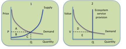
Figure 5: Demand and supply

In Figure 5 Panel 1, area ‘A’ represents the consumer surplus, which is the gain obtained by consumers because they are able to purchase a product at a market price that is less than the highest price they would be willing to pay (which is related to their benefit from consumption and represented by the demand curve). The producer surplus, depicted by ‘B’, is the amount that producers benefit by selling at a market price that is higher than the lowest price that they would be willing to sell for (which is related to their production costs and represented by the supply curve). The area ‘C’ represents production costs, which differ among producers and/or over the scale of production. The sum of areas A and B is labelled the ‘surplus’, and is interpreted as the net economic gain or welfare resulting from production and consumption with a quantity of Q at price P.

In the case that goods and services are not traded in a market (as is the case for many ecosystem services such as climate regulation, coastal protection and biodiversity), the interpretation of the welfare derived from their provision can also be represented in terms of surplus. Figure 5 Panel 2 represents the supply and demand of a non-marketed service. In this case, the service does not have a supply curve in the conventional sense that it represents the quantity of the service that producers are willing to supply at each price. The quantity of the service that is ‘supplied’ is not determined through a market at all but by other decisions regarding protection status, land use, management, access etc. The quantity of the service supplied is therefore independent of its value. This is represented in Figure 5 Panel 2 as a vertical line. The demand curve for non-marketed services is still represented as a downward sloping line since marginal benefits are expected to decline with quantity (the more that we have of a service, the lower the additional welfare of consuming more). In this case, consumers don’t pay a price for the quantity (Q) that is available to them and the entire area under the demand curve (D+E) represents their consumer surplus. It is useful to keep this Figure in mind when considering the measurement of service supply from an LME and the welfare people derive from it.

Note that the demand for goods and services that are used as inputs into the production of marketed goods and services (e.g., the habitat and nursery service provided to fisheries by mangroves and coastal wetlands are generally uncompensated inputs into fisheries production) is derived from the demand for the good or service that is finally consumed (e.g. fish).

The marginal value of a good or service is the contribution to wellbeing of one additional unit. It is equivalent to the price of the service in a perfectly functioning market (P in Figure 5). Small changes in ecosystem service provision should be valued using marginal values. The average value of a good or service can be calculated as its total value divided by the total quantity of the service provided and consumed. From Figure 5 Panel 2, average value can be calculated as (D+E)/Q. Average values may be useful for comparing the aggregate value of a good or service relative to the scale of provision (defined in terms of units of provision, area of ecosystem or number of beneficiaries).

Total Economic Value (TEV)

The concept of Total Economic Value (TEV) of an ecosystem is used to describe the comprehensive set of utilitarian values derived from that ecosystem. This concept is useful for identifying the different types of value that may be derived from an ecosystem. TEV comprises of use values and non-use values. Use values are the benefits that are derived from some physical use of the resource. Direct use values may derive from on-site extraction of resources (e.g. fisheries) or non-consumptive activities (e.g. recreation). Indirect use values are derived from off-site services that are related to the resource (e.g. climate regulation, coastal protection). Option value is the value that people place on maintaining the option to use an ecosystem resource in the future. Non-use values are derived from the knowledge that an ecosystem is maintained without regard to any current or future personal use. Non-use values may be related to altruism (maintaining an ecosystem for others), bequest (for future generations) and existence (preservation unrelated to any use) motivations. The constituent values of TEV are represented in Figure 6. It is important to understand that the “total” in Total Economic Value refers to the identification of all components of value rather than the sum of all value derived from a resource. TEV is a comprehensive measure, as opposed to a partial measure, of value. Accordingly, many estimates of TEV are for marginal changes in the provision of ecosystem services but “total” in the sense that they take a comprehensive view of sources of value.

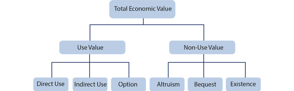
Figure 6: The components of Total Economic Value

The classification of different types of economic value within the concept of TEV is complementary to the classification of ecosystem services. Table 2 sets out the correspondence between categories of ecosystem service and components of TEV.

Table 2: Correspondence between ecosystem services and components of Total Economic Value

Exchange value

The concept of welfare value is used in most assessments of ecosystem services but it is not used in the System of National Accounts (SNA) that is used to calculate Gross Domestic Product (GDP) and other economic statistics. The SNA uses the concept exchange value, which is a measure of producer surplus plus the costs of production. In Figure 5 Panel 1 this is represented by areas B and C, or equivalently P times Q. Under the concept of exchange value, the total outlays by consumers and the total revenue of the producers are equal. For national accounting purposes, this approach to valuation enables a consistent and convenient recording of transactions between economic units since the values for supply and use of products are the same. In the context of comparing the values of ecosystem services with values in the system of national accounts, it is therefore necessary to value the total quantity of ecosystem services at the market prices that would have occurred if the services had been freely traded and exchanged. In other words, it is necessary to measure exchange value and not welfare value.

The differences between the concepts of welfare value and exchange value are the inclusion of consumer surplus (A) in the former and the inclusion of production costs in the latter (C). The concept of welfare value corresponds to a theoretically valid measure of welfare in the sense that a change in value represents a change in welfare for the producers and/or consumers of the goods and services under consideration. The concept of exchange value does not correspond to a theoretically valid measure of welfare and a change in exchange value does not necessarily represent a change in welfare for either producers or consumers (Day, 2013).2

2.4 Economic policy instruments

The term “policy instrument” is used to mean the mechanisms through which governments achieve a desired objective. Table 3 provides an overview of the main categories of environmental policy instrument. In general, economic policy instruments attempt to change the behaviour of stakeholders (e.g. consumers, fishers, resource users) by changing incentives that influence their decisions. Examples of economic policy instruments include taxes and subsidies, tradable permits or quotas, regulation of trade, and payments for ecosystem services. Chapter 8 provides detail on a number of policy instruments relevant to LME/MPA/ICM. The term “policy tool” on the other hand refers to frameworks, methodologies and models that can be used to inform policy making and the appraisal of policy instruments. Examples of economic policy tools include natural capital accounting (see chapter 7), cost-effectiveness analysis, cost-benefit analysis and multi-criteria analysis (see chapter 9).

Table 3. Classification of environmental policy instruments (UNEP 2007)